The Geography of Climate Adaptation
Geographic Heterogeneity in Climate Change Adaptation: Behavioral Evidence from Participation in Outdoor Activities
This research examines the role of non-market behavioral adaptation to climate change in the United States with a novel estimation procedure that accounts for both short-run weather and long-run climate adjustments. First, I comprehensively review the temperature sensitivity of all activities in the American Time Use Survey using a flexible non-linear estimation procedure. Most activities are found to be unresponsive to temperature with the exception of those that take place outdoors. These sensitive outdoor activities are studied further using the Climate Adaptation Response Estimation approach, which allows for temperature responses to vary geographically. The sensitivity to temperature varies across the country, and this variation is especially pronounced for cold-weather cities in which inhabitants reduce their outdoor and physical activities at extreme temperatures relative to warm-weather cities. Finally I forecast the expected change in outdoor activity time using climate models compiled by the Intergovernmental Panel on Climate Change, finding a large increase in outdoor time driven by warmer winters.
Download with figures embedded in the text or with figures following the text.
The Great Outdoors
Lockdowns across the world in 2020 during the COVID-19 crisis have demonstrated the importance of spending time outdoors. Mental and physical health outcomes improve in natural environments. The figure below shows the share of time spent during different activities where the primary emotion was negative (e.g. a person felt more tired than alert or felt more depressed than happy):
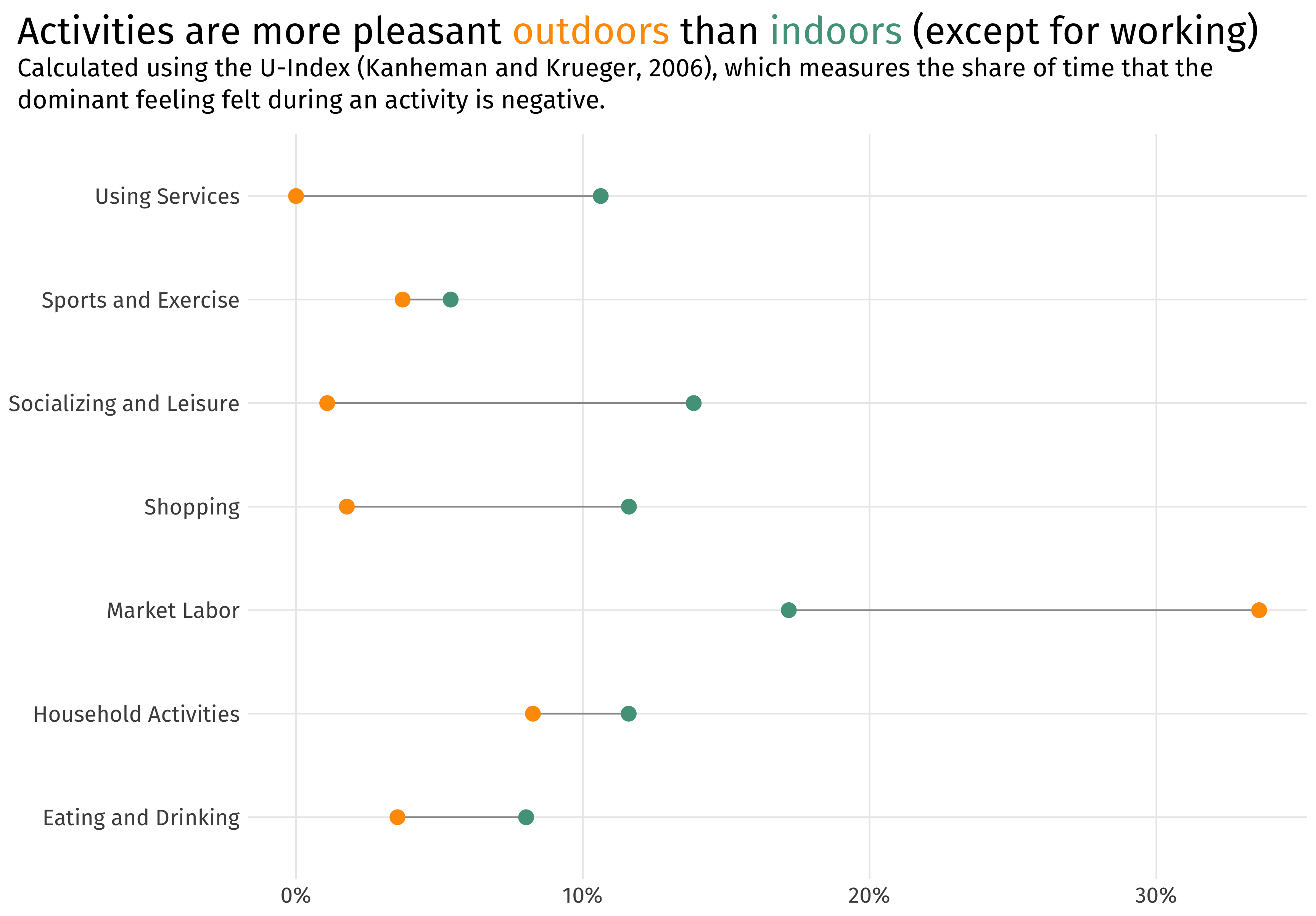
Clearly spending time outside is more pleasant than inside during non-labor activities. Despite the importance of time outdoors, future climate change threatens the way people allocate time outside in ways that we don’t understand. This research estimates communities’ sensitivities to temperature and how these sensitivities vary across the United States due to the local climate.
To demonstrate the geographic heterogeneity in temperature sensitivity, the animation below plots the average share of the day spent outside in each state using data from the American Time Use Survey: 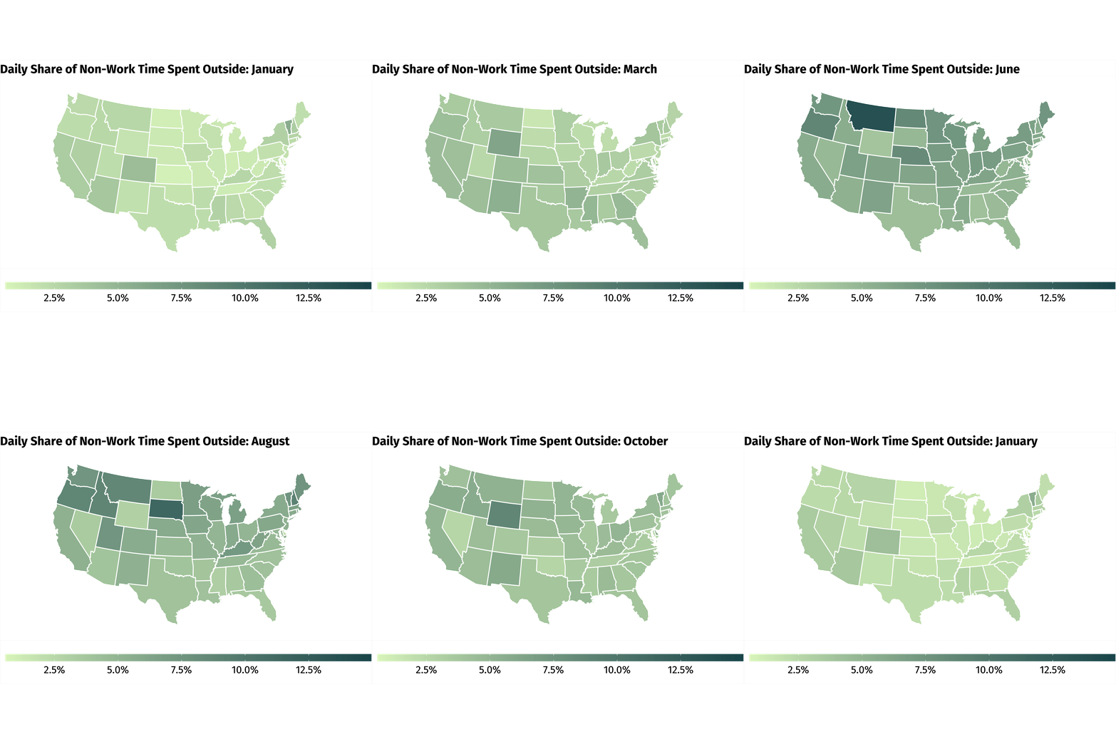
We see the expected seasonality – people spend more time outside during the late spring and summer than in the winter – but we also see some clear differences across states. What’s driving this heterogeneity?
The Sensitivity to Weather
Not all states are equally amenable to spending time outside. We wouldn’t expect to be outdoors for long periods during a January in Chicago or a July in Austin. In order to assess the sensitivity to weather, I estimate a semi-parametric temperature response function for each metropolitan area in the country. Doing so gives us a better understanding of how people react to different ranges of temperatures. The model can be represented as:
\[y_{it} = \sum_{b \in B \backslash \{60-70\}} \beta_{b} D_{ibt} + \gamma X_{ijt} + \alpha_{jm} + \phi_{my} + \epsilon_{it}\]where $y_{it}$ represents the number of minutes respondent $i$ spent doing activity $y$ at time $t$ and $D_{ibt}$ is an indicator for whether the temperature experienced by respondent $i$ at time $t$ falls into temperature bin $b$. The model allows for non-linearities in the temperature-outcome relationship by including these indicators. $X_{ijt}$ is a vector of confounding variables which are adjusted for, including other weather variables (precipitation, humidity, and wind speed), demographic characteristics of respondent $i$ from the Current Population Survey (age, race, marital status, number of children, education, household income, home ownership status), ATUS diary information (day of the week the diary was completed for, an indicator for whether the diary day was a holiday) and region $j$ geographic and economic characteristics (elevation, slope, air conditioning prevalence). $\alpha_{jm}$ are region-month fixed effects and $\phi_{my}$ are month-year fixed effects. The set of fixed effects absorb unobserved region-month and month-year determinants of time allocation.
The graph below plots the estimated coefficients for each 10-degree Farenheit temperature bin. The coefficients are relative to a baseline temperature of 60-70 degrees, so they can be interpreted as the change in the number of minutes spent outdoors each as a result of the day being in a particular temperature bin instead of the 60-70 degree bin. For reference, the unconditional mean number of minutes spent outdoors per day in the American Time Use Survey is 31.4 and, conditional on spending some time outside, the mean is 93.4 minutes.
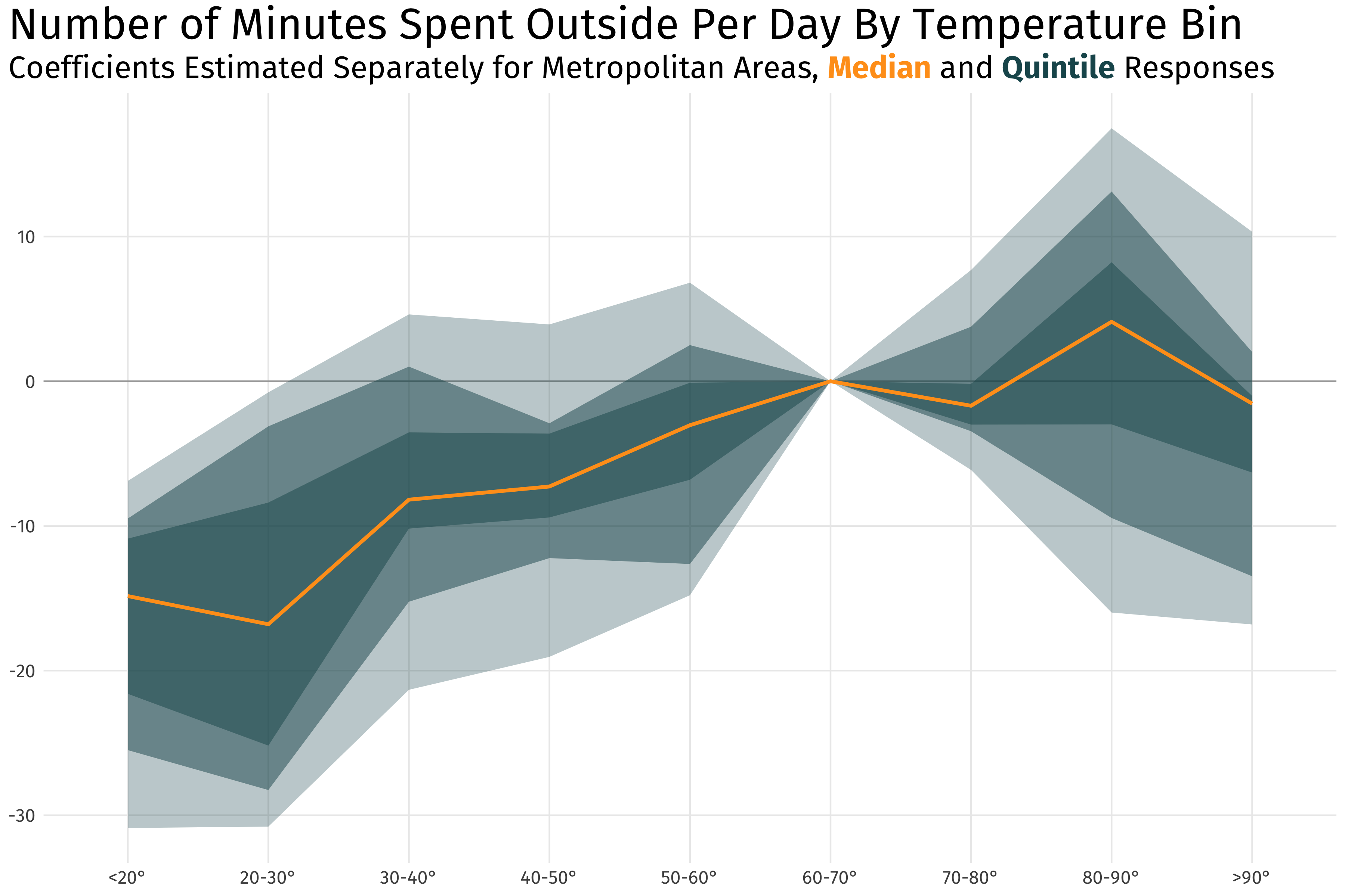
The key takeaway is that most cities are very sensitive to cold temperatures and not very sensitive to hot temperatures. However the effect is not uniform across all the cities in the sample. The effect is large, especially in the most extreme temperature bins, where there is roughly a 50% decrease in time outside. Importantly, these results estimate the short-run weather response, not the long-run climate response. In order to understand how the local climate influences the estimated temperature sensitivities, we need to go one step further.
The Climate Effect
Even though we might not expect to spend much time outside during a Chicago winter, the average Austin winter is more amenable to outdoor activities. By the same logic, Chicagoans are likely more prepared for cold weather days regardless of the time of year. That is, Chicagoans have adapted to their local climate through investments in cold-climate infrastructure which make those extreme cold days more bearable. Restaurants in Chicago, for example, are largely well insulated. The same cannot be said of Austin’s food trucks.
So how much do these sorts of long-run climate investments affect the amount of time people spend outdoors? In order to estimate the climate effect on outdoor time, I regress the coefficients from the previous graph on the share of days a city experiences in all the temperature bins from 1979-2004. Plainly, I calculate how much the slope of the previous graph is affected by the local long-run climate.
The figure below plots the change in the temperature response slope due to the share of days in the cold and warm temperature bins for two synthetic cities, one cold and one hot. Other than the average annual temperature, the two synthetic cities are identical in terms of their income, population density, and share of greenspace – all factors that may influence how they respond to temperature.
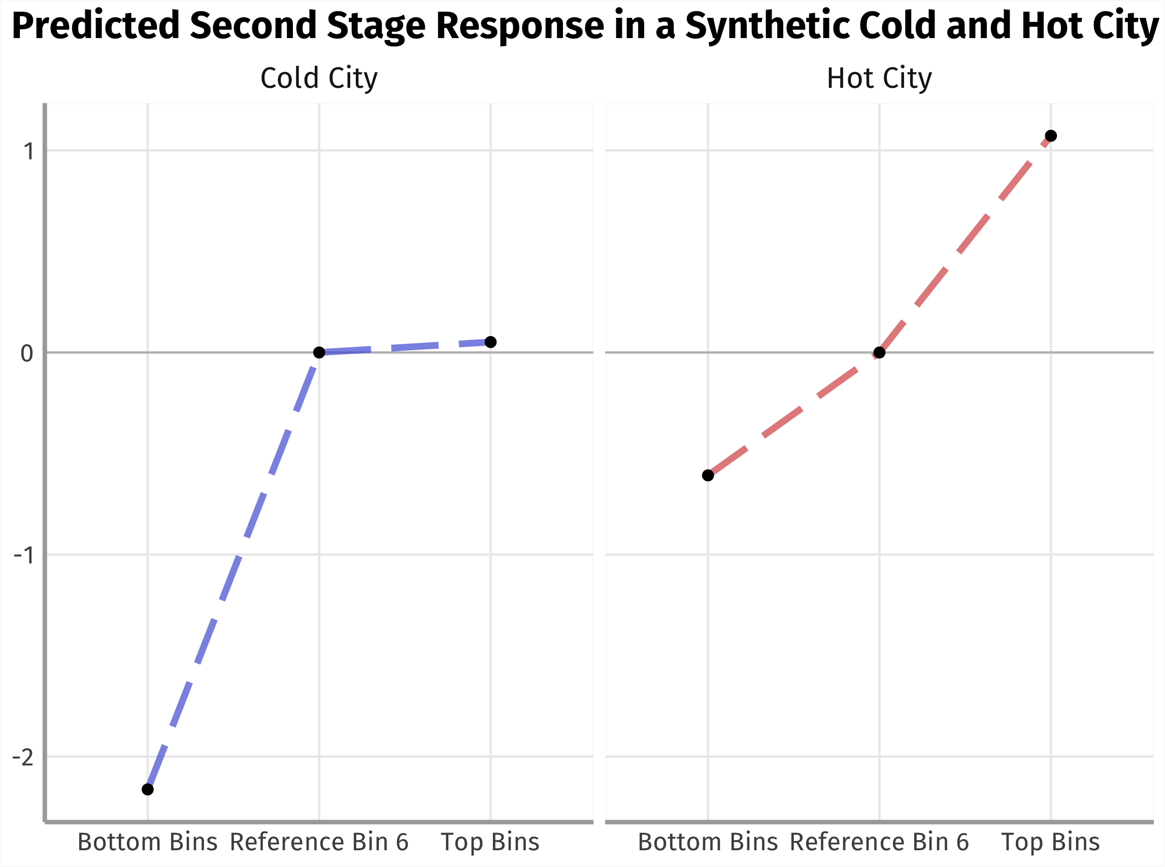
Both the hot and cold city respond negatively to the share of cold days, but the cold weather cities are especially responsive. For reference, a predicted value of -2 represents nearly 10% of the total effect from the coefficients from the previous graph. The response to hot climate is more measured, suggesting limited ability to adapt relative to cold weather adaptation.
The Climate Forecast and Its Implications
Having established that cities in the U.S. are very sensitive to cold temperatures and the sensitivities are especially pronounced in cities that frequently experience cold days, I can now forecast how climate change at the end of the century will affect the amount of time we spend outside.
The graph below plots the change in the number of days that fall in 5-degree temperature bins under three different climate scenarios published by the Intergovernmental Panel on Climate Change.
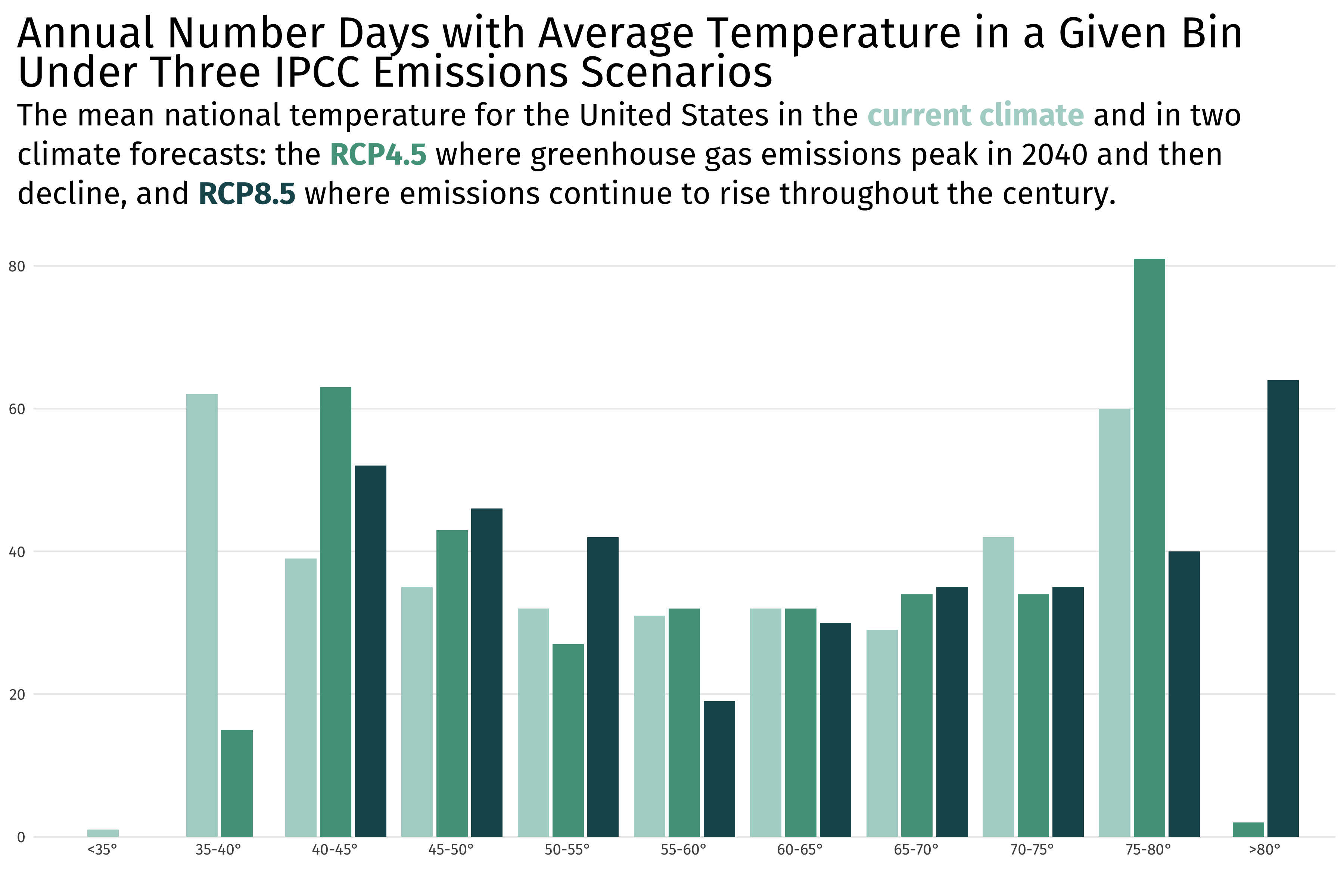
As we would expect, more greenhouse gas emissions lead to large rightward shifts in the temperature distribution. At the city level, the implication is that people will adjust the amount of time they spend outdoors because the number of pleasant days has changed. How much they adjust will depend on where they live:
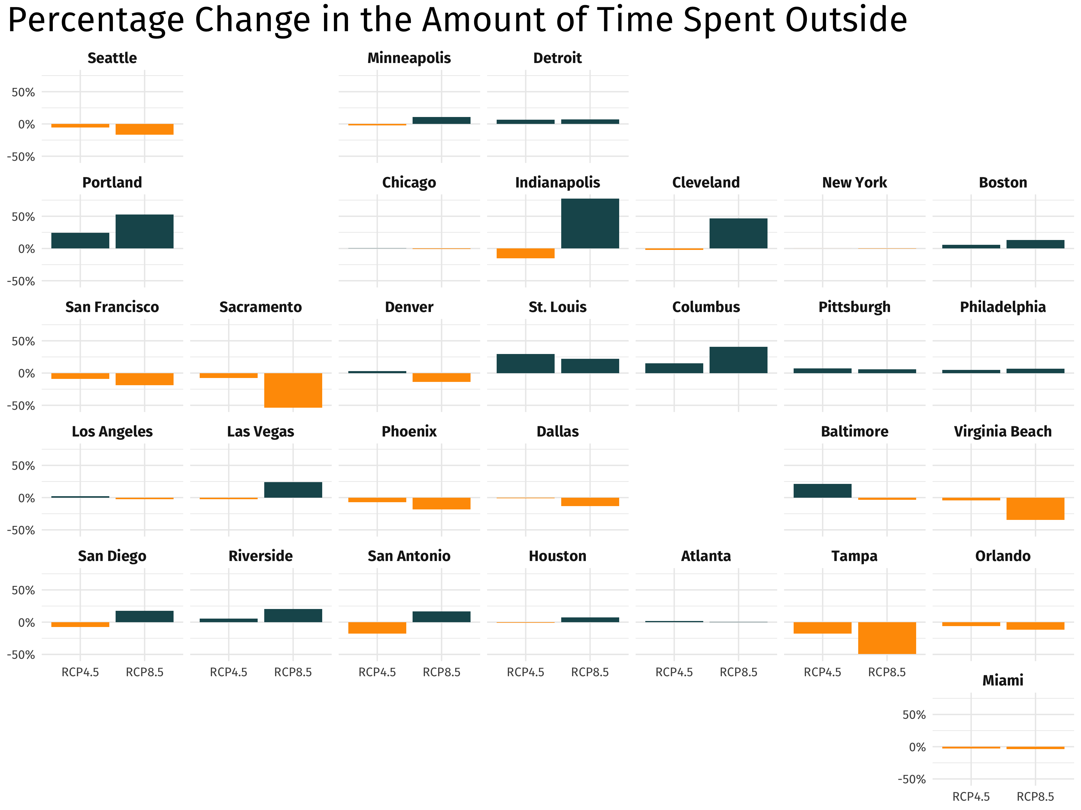
In general cities in the North see substantial increases in the amount of time people will spend outside due to warmer winters, but Southern cities will see similar decreases due to warmer summers. Finally, I estimate the expected welfare effects that result from the change in outdoor time. Returning to the U-Index from the first figure, I forecast the expected change in time spent doing unpleasant activities as a result of climate change.
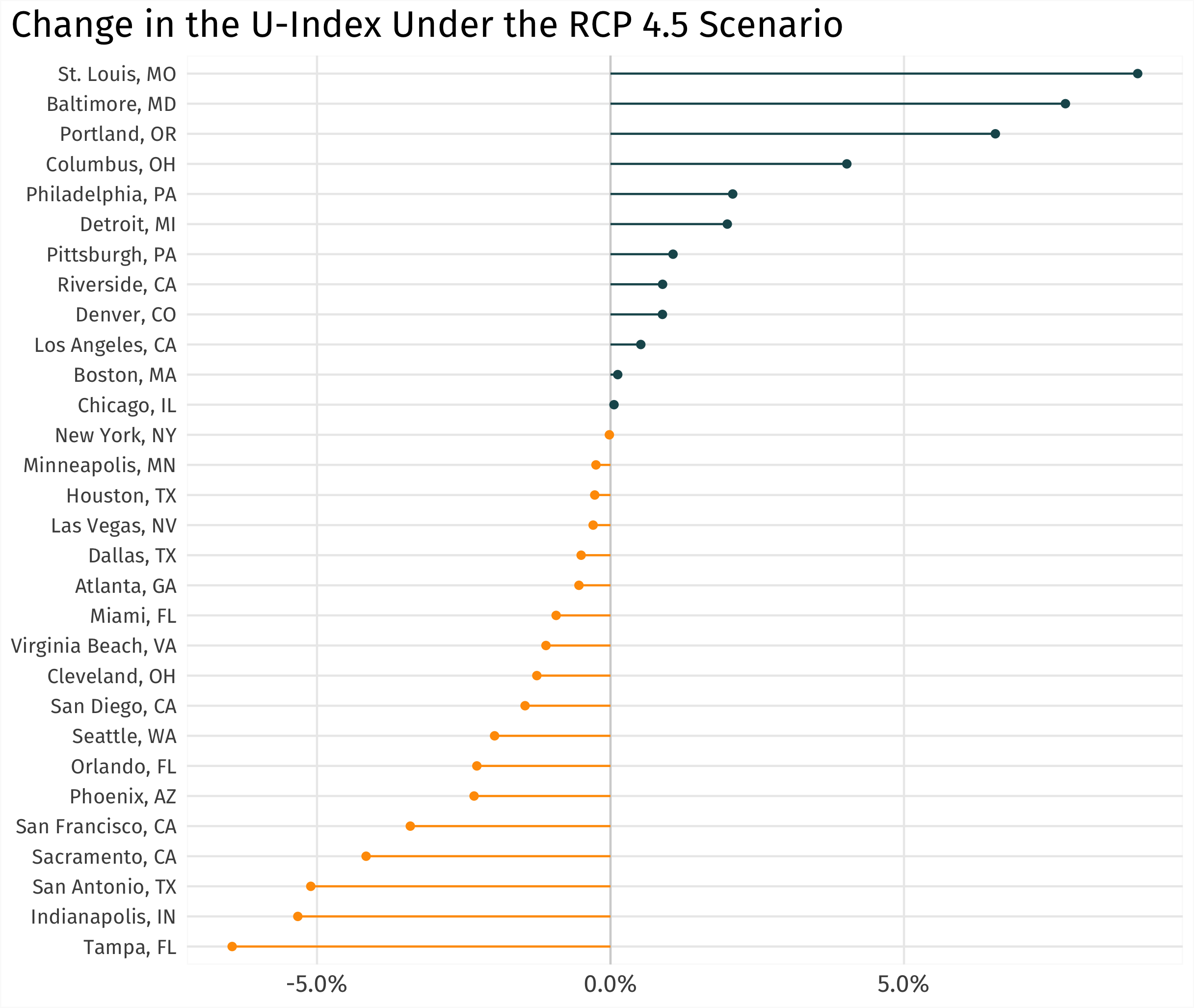
The forecasted welfare change as a result of climate change depends largely on where a person lives. For investors and policymakers, overlooked vectors of behavioral change due to climate change like the amount of time spent outdoors could have profound impacts on the welfare of the public and these impacts are not uniform across the country. Further research should carefully consider how the long-run climate of a city or country will affect how that place responds to climate change.
